A while ago, I was a TA in the Data Structures course at uOttawa and I got the assignment of designing a tutorial about hash tables in Java. Although I was familiar with the concept, nevertheless I had to do some reading to gain a better understanding of the material and deliver a successful presentation.
A hash table is a common data structure present in almost any language. The main ideas introduced by this structure are:
- The use of hash function to map general keys to corresponding indices in an array of bucket (slots).
- The use of collision-handling schemes to address the problem of two different keys mapping to the same index.
- Provides an amortized constant average cost per operations such as insert, find and delete. For a more in-depth explanation, check the Wikipedia page or read any introductory book in data structures :D.
Now, building from that experience, I decided to focus on adding a HashTable implementation to the DataStructures101 gem.
For this first part, we are only going to focus in the analysis of the essential concepts of a hash table.
Hash Functions
Based on the idea mentioned above, we can define a hash function as a function h that maps a given key k to an integer in the range [0, N - 1], where N is the capacity of the bucket array.
In an ideal world, our hash function would make sure that each key corresponds to a different integer. But in reality, sometimes happens that two (or more) different keys produce the same integer index, which means these keys are going to be mapped to the same bucket in our hash table. In situation like this, we are in presence of what is known as a collision. We’ll see later some strategies to deal with collisions, but the best approach is to try to avoid them at all. For this, we always should strive to use a “good” hash function, good meaning that it should minimize the number of collisions between the set of keys, as well as being fast and easy to compute.
To facilitate our understanding (and our future implementation), we are going to view our hash function h(k) as being made of two different operations:
- Hash code: Which maps a key k to an integer, and
- Compression function: Which maps a hash code hc to the range [0, N - 1].
The main advantage of this separation is that computation of the hash code can be made independent of the specific table size, allowing for the general hash code computation of objects for any hash table size.
Hash Codes
To formalize our understanding of a hash code, we can say that an object hash code is w-bit integer number and for any two x and y codes the following properties should hold:
- If x and y are equal, then
x.hash_codeequalsy.hash_code. - If x and y are not equal, then the probability that
x.hash_codeis equal toy.hash_codeshould be as smaller as possible.
The first property ensures that we are capable of finding everytime the object x after insertion in our hash table. The second one, minimizes the information loss of converting random objects into integers, by ensuring that different objects usually have different hash codes.
Based on this properties, we desire our hash code function to produce a set of keys that minimizes the number of collisions as much as possible, otherwise our compression function won’t be capable to avoid them. Below, we discuss some practical and common hash codes implementations.
Bit Representation
For any primitive data type (i.e. integers, float, char, bytes, etc..), we can simply use as hash code an integer interpretation of the bits, as long as the number of bits is no larger that number of bits in our hash code.
If our object type has a longer bit representation (such as long or double type), then the previous approach is not directly applicable. To solve it, we can either take the high-order bits (or low-order bits) that fit our integer representation; or we can combine all the original bits through bit operations to fit the hash code size. Taking the high-order (low-order) bits usually leads to collision if the set of keys mostly differs in the bit portion that we are throwing away, so bit operations such as the exclusive-or or an overflow addition of the numbers tend to yield better results.
Polynomial Hash Codes
If we want to generate the hash code for a variable-length object (e.g. a string), using bit representation may not be the best solution to use. This usually due to significance of the order of the elements in the object.
Instead, if we consider the object as a tuple of the form $$ (x_0,x_1,…,x_{n-1})$$ where each \(x_i\) correspond to an element in the object, then we can take into consideration each of the different positions by using as hash code the following polynom: $$x_0a^{n-1}+x_1a^{n-2}+…+x_{n-2}a+x_{n-1}$$ where a is an integer constant such that \(a \ne 0\) and \(a \ne 1\).
Intuitively, a polynomial hash code will spread out the influence of each element in the component across the resulting hash code.
Common values for a are 33, 37, 39 and 41 (particularly when working with character strings that are English words).
Cyclic-Shift Hash Codes
Cyclic-Shift is a variation of the polynomial hash code. Instead of doing a multiplication by a constant a value, it performs a cyclic shift of a partial sum by a certain amount of bits. Sounds difficult? Nah!
For example, a 4-bit cycle left shift of the 8 bit value 11100000 is achieved by removing the 4 leftmost bits and placing them at the rightmost side of the bit representation, which results in 00001110.
Although this process does not mean much in arithmetics, it has the property of varying the bits of the calculation.
Compression Functions
The hash code resulting of the application of the previous mentioned methods will typically not be suitable for direct use with a bucket array, because the integer hash may be negative or be larger than the capacity of the bucket array. Thus, we still have to solve the issue of fitting our hash code within the range \([0, N - 1]\). This computation, named compression function is the second action performed by the overall hash function.
Division Method
The division method is a simple compression function, which maps an integer i to $$i\; mod\; N$$ where N is the size of the bucket array. Usually N is taken as prime number, to help spread out the distribution of hashed values.
MAD Method
The MAD method, which stands for Multiply-Add-and-Divide is a more sophisticated compression function, that maps an integer i using the following approach: $$[(ai + b)\; mod\; p]\; mod\; N$$ where once again, N is the size of the bucket array, p is a prime number larger that \(N\) and a and b are random integers from the interval [0, p - 1], with \(a \gt 0\).
Collision-handling Schemes
So far, we have accomplished generating hash codes for any key fitting in the range of \([0, N - 1]\). In the following subsections we are going to discuss different techniques to solve the remaining issue: how to deal with two distinct keys \(k_1\) and \(k_2\) that map to the same location in the bucket array (a collision). These collisions prevent to insert directly a new entry \((k,v)\) directly into the bucket array at position \(h(k)\).
Separate Chaining
A simple way to handle collisions is to each bucket to store its own container (e.g., a list), which will hold all the instances of keys that were mapped to the same hash code, as shown in the image below.
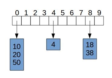
On an individual bucket, operations are going to perform proportional to the size of the bucket. Assuming we have a “good” hash function and we are indexing n entries in the hash table, it would be expected that the core operations run in \(O(\lceil n/N \rceil)\). The closer this ratio is to \(O(1)\) the better performance our implementation will have.
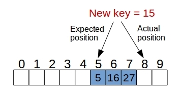
Linear Probing
Linear probing is one the simple methods of the family of open addressing schemes (which refers to the collision-handling schemes that store each entry directly in a table slot, thus saving memory space by not using an extra data structure).
With this approach, if we proceed to insert an entry (k,v) into a bucket at position \(j = h(k)\) that is already occupied, then we proceed to iterate over \(A[(j + i)\; mod\; N]\) for \(i = 0,1,2..\) until we find an empty slot to insert the new entry, as shown in the following diagram.
Of course this introduces several changes in the implementation to search for a given key, because now in order to locate a key k we may have to examine several consecutive slots starting from \(A[h(k)]\) until we find an entry with the same key or we find an empty slot. For deletion, we cannot simple remove the entry from the table, because it could other valid searches to fail because we found an empty slot, so a common solution it is to use a predetermined valid to mark those slots as special empty.
Quadratic Probing
A variantion of the linear probing scheme, it iteratively tries the buckets \(A[(h(k) + f(i))\; mod\; N\), for \(i = 0,1,2…\), where \(f(i) = i^2\) until it finds an empty slot.
This strategy still has to deal with a more complicated deletion process, as in linear probing, but it avoids the clustering patterns of consecutive slots introduced by the former. Nevertheless, it brings its own issues, mainly that can only guarantee insertion if the the table is less than half full and the \(N\) is chosen to be prime, and the introduction of its own type of clustering of keys, usually called secondary clustering.
Double Hashing
Another open addressing strategy, double hashing avoids the former clustering issues by choosing a secondary hash function \(h^{'}\). It works by iteratively analyzing the slots of the form \(A[((h(k) + f(i))\; mod\;N]\) for \(i = 0,1,2..\), where \(f(i) = i \times h^{'}(k)\) until it finds the first one empty. It is important to note that in this scheme the secondary hash function cannot evaluate to zero; a common choice is \(h^{'}(k) = q - (k\;mod\;q)\) for some prime number \(q \lt N\). N should be prime as well.
This one was a long post. Uff!! Thankfully, by now we have finish with the more boring and conceptual stuff :). Next post will have all the goodies related to how we implement these features in a HashTable class in Ruby.
To sum it up, thanks to read till the very end and hope it has been worth to you. See you soon again and stay tuned for more!!